
Videos
Develop a spreadsheet for computing the demand for any values of the input variables in the linear demand and nonlinear demand prediction models in Examples
To develop a spreadsheet for computing the demand for any values if the input variables in the linear demand and nonlinear demand prediction models.
Explanation of Solution
Given:
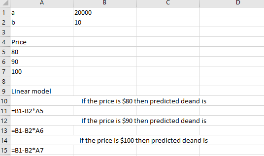
Linear model is,
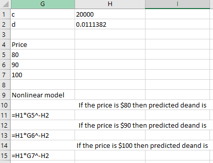
And Nonlinear model,
Following is the formulae used in spreadsheet for linear model:
Following is the formulae used in spreadsheet for Nonlinear model:
Following is the output for linear model:
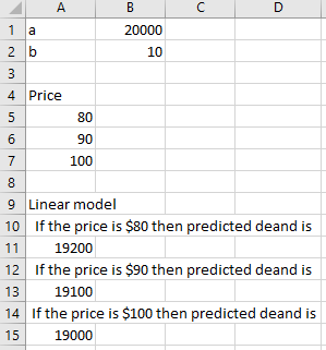
As per calculation, if the price increases then demand decreases.
Following is the output for Nonlinear model:
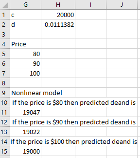
As per calculation, if the price increases then demand decreases.
Want to see more full solutions like this?
Chapter A1 Solutions
Business Analytics
Additional Math Textbook Solutions
APPLIED STAT.IN BUS.+ECONOMICS
Statistical Reasoning for Everyday Life (5th Edition)
Statistics: Informed Decisions Using Data (5th Edition)
Statistics Through Applications
Elementary Statistics (Text Only)
Elementary Statistics: A Step By Step Approach


- Sometimes curvature in a scatterplot can be fit adequately (especially to the naked eye) by several trend lines. We discussed the exponential trend line, and the power trend line is discussed in the previous problem. Still another fairly simple trend line is the parabola, a polynomial of order 2 (also called a quadratic). For the demand-price data in the file P13_10.xlsx, fit all three of these types of trend lines to the data, and calculate the MAPE for each. Which provides the best fit? (Hint: Note that a polynomial of order 2 is still another of Excels Trend line options.)arrow_forwardDilberts Department Store is trying to determine how many Hanson T-shirts to order. Currently the shirts are sold for 21, but at later dates the shirts will be offered at a 10% discount, then a 20% discount, then a 40% discount, then a 50% discount, and finally a 60% discount. Demand at the full price of 21 is believed to be normally distributed with mean 1800 and standard deviation 360. Demand at various discounts is assumed to be a multiple of full-price demand. These multiples, for discounts of 10%, 20%, 40%, 50%, and 60% are, respectively, 0.4, 0.7, 1.1, 2, and 50. For example, if full-price demand is 2500, then at a 10% discount customers would be willing to buy 1000 T-shirts. The unit cost of purchasing T-shirts depends on the number of T-shirts ordered, as shown in the file P10_36.xlsx. Use simulation to determine how many T-shirts the company should order. Model the problem so that the company first orders some quantity of T-shirts, then discounts deeper and deeper, as necessary, to sell all of the shirts.arrow_forwardSuppose that a regional express delivery service company wants to estimate the cost of shipping a package (Y) as a function of cargo type, where cargo type includes the following possibilities: fragile, semifragile, and durable. Costs for 15 randomly chosen packages of approximately the same weight and same distance shipped, but of different cargo types, are provided in the file P13_16.xlsx. a. Estimate a regression equation using the given sample data, and interpret the estimated regression coefficients. b. According to the estimated regression equation, which cargo type is the most costly to ship? Which cargo type is the least costly to ship? c. How well does the estimated equation fit the given sample data? How might the fit be improved? d. Given the estimated regression equation, predict the cost of shipping a package with semifragile cargo.arrow_forward
- When you use a RISKSIMTABLE function for a decision variable, such as the order quantity in the Walton model, explain how this provides a fair comparison across the different values tested.arrow_forwardPlay Things is developing a new Lady Gaga doll. The company has made the following assumptions: The doll will sell for a random number of years from 1 to 10. Each of these 10 possibilities is equally likely. At the beginning of year 1, the potential market for the doll is two million. The potential market grows by an average of 4% per year. The company is 95% sure that the growth in the potential market during any year will be between 2.5% and 5.5%. It uses a normal distribution to model this. The company believes its share of the potential market during year 1 will be at worst 30%, most likely 50%, and at best 60%. It uses a triangular distribution to model this. The variable cost of producing a doll during year 1 has a triangular distribution with parameters 15, 17, and 20. The current selling price is 45. Each year, the variable cost of producing the doll will increase by an amount that is triangularly distributed with parameters 2.5%, 3%, and 3.5%. You can assume that once this change is generated, it will be the same for each year. You can also assume that the company will change its selling price by the same percentage each year. The fixed cost of developing the doll (which is incurred right away, at time 0) has a triangular distribution with parameters 5 million, 7.5 million, and 12 million. Right now there is one competitor in the market. During each year that begins with four or fewer competitors, there is a 25% chance that a new competitor will enter the market. Year t sales (for t 1) are determined as follows. Suppose that at the end of year t 1, n competitors are present (including Play Things). Then during year t, a fraction 0.9 0.1n of the company's loyal customers (last year's purchasers) will buy a doll from Play Things this year, and a fraction 0.2 0.04n of customers currently in the market ho did not purchase a doll last year will purchase a doll from Play Things this year. Adding these two provides the mean sales for this year. Then the actual sales this year is normally distributed with this mean and standard deviation equal to 7.5% of the mean. a. Use @RISK to estimate the expected NPV of this project. b. Use the percentiles in @ RISKs output to find an interval such that you are 95% certain that the companys actual NPV will be within this interval.arrow_forwardThe Baker Company wants to develop a budget to predict how overhead costs vary with activity levels. Management is trying to decide whether direct labor hours (DLH) or units produced is the better measure of activity for the firm. Monthly data for the preceding 24 months appear in the file P13_40.xlsx. Use regression analysis to determine which measure, DLH or Units (or both), should be used for the budget. How would the regression equation be used to obtain the budget for the firms overhead costs?arrow_forward
- A company manufacturers a product in the United States and sells it in England. The unit cost of manufacturing is 50. The current exchange rate (dollars per pound) is 1.221. The demand function, which indicates how many units the company can sell in England as a function of price (in pounds) is of the power type, with constant 27556759 and exponent 2.4. a. Develop a model for the companys profit (in dollars) as a function of the price it charges (in pounds). Then use a data table to find the profit-maximizing price to the nearest pound. b. If the exchange rate varies from its current value, does the profit-maximizing price increase or decrease? Does the maximum profit increase or decrease?arrow_forwardThe file P13_22.xlsx contains total monthly U.S. retail sales data. While holding out the final six months of observations for validation purposes, use the method of moving averages with a carefully chosen span to forecast U.S. retail sales in the next year. Comment on the performance of your model. What makes this time series more challenging to forecast?arrow_forwardAn automobile manufacturer is considering whether to introduce a new model called the Racer. The profitability of the Racer depends on the following factors: The fixed cost of developing the Racer is triangularly distributed with parameters 3, 4, and 5, all in billions. Year 1 sales are normally distributed with mean 200,000 and standard deviation 50,000. Year 2 sales are normally distributed with mean equal to actual year 1 sales and standard deviation 50,000. Year 3 sales are normally distributed with mean equal to actual year 2 sales and standard deviation 50,000. The selling price in year 1 is 25,000. The year 2 selling price will be 1.05[year 1 price + 50 (% diff1)] where % diff1 is the number of percentage points by which actual year 1 sales differ from expected year 1 sales. The 1.05 factor accounts for inflation. For example, if the year 1 sales figure is 180,000, which is 10 percentage points below the expected year 1 sales, then the year 2 price will be 1.05[25,000 + 50( 10)] = 25,725. Similarly, the year 3 price will be 1.05[year 2 price + 50(% diff2)] where % diff2 is the percentage by which actual year 2 sales differ from expected year 2 sales. The variable cost in year 1 is triangularly distributed with parameters 10,000, 12,000, and 15,000, and it is assumed to increase by 5% each year. Your goal is to estimate the NPV of the new car during its first three years. Assume that the company is able to produce exactly as many cars as it can sell. Also, assume that cash flows are discounted at 10%. Simulate 1000 trials to estimate the mean and standard deviation of the NPV for the first three years of sales. Also, determine an interval such that you are 95% certain that the NPV of the Racer during its first three years of operation will be within this interval.arrow_forward
- In Problem 12 of the previous section, suppose that the demand for cars is normally distributed with mean 100 and standard deviation 15. Use @RISK to determine the best order quantityin this case, the one with the largest mean profit. Using the statistics and/or graphs from @RISK, discuss whether this order quantity would be considered best by the car dealer. (The point is that a decision maker can use more than just mean profit in making a decision.)arrow_forwardUse @RISK to analyze the sweatshirt situation in Problem 14 of the previous section. Do this for the discrete distributions given in the problem. Then do it for normal distributions. For the normal case, assume that the regular demand is normally distributed with mean 9800 and standard deviation 1300 and that the demand at the reduced price is normally distributed with mean 3800 and standard deviation 1400.arrow_forwardNorth Dakota Electric Company estimates its demand trend line (in millions of kilowatt hours) to be: D = 80.0 + 0.50Q, where Q refers to the sequential quarter number and Q = 1 for winter of Year 1. In addition, the multiplicative seasonal factors are as follows: Quarter Factor (Index) Winter 0.80 Spring 1.25 Summer 1.50 Fall 0.45 In year 26 (quarters 101-104), the energy use for each of the quarters beginning with winter is (round your response to one decimal place): Quarter Energy Use Winter Spring Summer Fallarrow_forward
 Practical Management ScienceOperations ManagementISBN:9781337406659Author:WINSTON, Wayne L.Publisher:Cengage,