Chapter 1, Problem 40E

(Exercises 27–40) For each description of data, identify the W’s, name the variables, specify for each variable whether its use indicates that it should be treated as categorical or quantitative, and, for any quantitative variable, identify the units in which it was measured (or note that they were not provided).

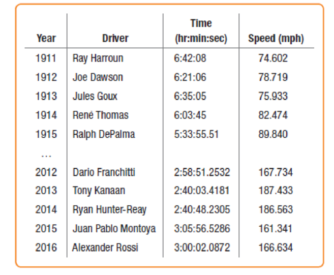
40. Indy 500 2016 The 2.5-mile Indianapolis Motor Speedway has been the home to a race on Memorial Day nearly every year since 1911. Even during the first race, there were controversies. Ralph Mulford was given the checkered flag first but took three extra laps just to make sure he’d completed 500 miles. When he finished, another driver, Ray Harroun, was being presented with the winner’s trophy, and Mulford’s protests were ignored. Harroun averaged 74.6 mph for the 500 miles. In 2013, the winner, Tony Kanaan, averaged over 187 mph, beating the previous record by over 17 mph!

Here are the data for the first five races and five recent Indianapolis 500 races.