
Sub part (a):
Consumption schedule and marginal propensity to consume.
Sub part (a):
Explanation of Solution
Table -1 shows the consumption schedule:
Table -1
|
| Consumption |
| 100 | 120 |
| 200 | 200 |
| 300 | 280 |
| 400 | 360 |
| 500 | 440 |
| 600 | 520 |
| 700 | 600 |
Figure 1 illustrates the level of consumption at different level of gross domestic product (GDP).
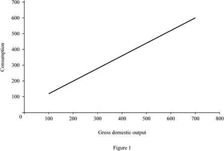
In Figure 1, the horizontal axis measures the gross domestic output and the vertical axis measures the consumption level.
Size of marginal propensity to consume (MPC) can be calculated as follows.
The size of marginal propensity to consume is 0.8.
Concept introduction:
Consumption schedule: Consumption schedule refers to the quantity of consumption at different levels of income.
Marginal propensity to consume (MPS): Marginal propensity to consume refers to the sensitivity of change in the consumption level due to the changes occurred in the income level.
Sub part (b):
Disposable income, tax rate, consumption schedule, marginal propensity to consume and multiplier.
Sub part (b):
Explanation of Solution
Disposable income (DI) can be calculated by using the following formula.
Substitute the respective values in Equation (1) to calculate the disposable income at the level of GDP $100.
Disposable income at the level of GDP $100 is $90.
Tax rate can be calculated by using the following formula.
Substitute the respective values in Equation (2) to calculate the tax rate at the level of GDP $100.
Tax rate at the level of GDP is 10%.
New consumption level can be calculated by using the following formula.
Substitute the respective values in Equation (3) to calculate the disposable income at the level of GDP $100. Since, the tax payment is equal amount of decrease in consumption for all the levels of GDP. The decreasing consumption for increasing $10 is assumed to be $8.
New consumption is $112.
Table -2 shows the values of disposable income, new consumption level after tax and the tax rate that are obtained by using Equations (1), (2) and (3).
Table -2
| Gross domestic product | Tax | DI | New consumption | Tax rate |
| 100 | 10 | 90 | 112 | 10% |
| 200 | 10 | 190 | 192 | 5% |
| 300 | 10 | 290 | 272 | 3.33% |
| 400 | 10 | 390 | 352 | 2.5% |
| 500 | 10 | 490 | 432 | 2% |
| 600 | 10 | 590 | 512 | 1.67% |
| 700 | 10 | 690 | 592 | 1.43% |
Size of marginal propensity to consume (MPC) can be calculated as follows.
The size of marginal propensity to consume is 0.8.
Multiplier: Multiplier refers to the ratio of change in the real GDP to the change in initial consumption, at a constant price rate. Multiplier is positively related to the marginal propensity to consumer and negatively related with the marginal propensity to save. Multiplier can be evaluated using the following formula:
Since the value of MPC remains the same for part (a) and part (b), there is no change in the value of multiplier. The value of multiplier is 5
Figure -2 illustrates the level of consumption at different level of gross domestic product (GDP) for lump sum tax (Regressive tax).
In Figure -2, the horizontal axis measures the gross domestic output and the vertical axis measures the consumption level.
Concept introduction:
Consumption schedule: Consumption schedule refers to the quantity of consumption at different levels of income.
Marginal propensity to consume (MPS): Marginal propensity to consume refers to the sensitivity of change in the consumption level due to the changes occurred in the income level.
Multiplier: Multiplier refers to the ratio of change in the real GDP to the change in initial consumption at constant price rate. Multiplier is positively related to the marginal propensity to consumer and negatively related with the marginal propensity to save.
Sub part (c):
Tax amount, consumption schedule, marginal propensity to consume and multiplier.
Sub part (c):
Explanation of Solution
Tax amount can be calculated by using the following formula.
Substitute the respective values in Equation (4) to calculate the tax amount at $100 GDP.
Tax amount is $10.
Table -3 shows the values of disposable income, new consumption level after tax and the tax rate that are obtained by using Equations (1), (2), (3) and (4). The change in tax amount is differing for different levels of GDP. The decreasing consumption for increasing each $10 is assumed to be $8 (Thus, if the tax payment is $30, then the consumption decreases by $24
Table -3
| Gross domestic product | Tax | DI | New consumption | Tax rate |
| 100 | 10 | 90 | 112 | 10% |
| 200 | 20 | 180 | 184 | 10% |
| 300 | 30 | 270 | 256 | 10% |
| 400 | 40 | 360 | 328 | 10% |
| 500 | 50 | 450 | 400 | 10% |
| 600 | 60 | 540 | 472 | 10% |
| 700 | 70 | 630 | 544 | 10% |
Multiplier: Multiplier refers to the ratio of change in the real GDP to the change in initial consumption, at a constant price rate. Multiplier is positively related to the marginal propensity to consumer and negatively related with the marginal propensity to save. Multiplier can be evaluated using the following formula:
Since the value of MPC different for part (a) and part (c), the value of multiplier for both the part is different. The value of multiplier is 3.57
Figure -3 illustrates the level of consumption at different level of gross domestic product (GDP) for proportional tax.
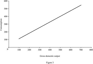
In Figure -3, the horizontal axis measures the gross domestic output and the vertical axis measures the consumption level.
Concept introduction:
Consumption schedule: Consumption schedule refers to the quantity of consumption at different levels of income.
Marginal propensity to consume (MPS): Marginal propensity to consume refers to the sensitivity of change in the consumption level due to the changes occurred in the income level.
Multiplier: Multiplier refers to the ratio of change in the real GDP to the change in initial consumption at constant price rate. Multiplier is positively related to the marginal propensity to consumer and negatively related with the marginal propensity to save.
Sub part (d):
consumption schedule, marginal propensity to consume and multiplier.
Sub part (d):
Explanation of Solution
Marginal propensity to consume can be calculated by using the following formula.
Substitute the respective values in Equation (5) to calculate the MPC at $100 GDP.
The value of MPC is 0.72.
Table -4 shows the values of disposable income, new consumption level after tax and the tax rate that are obtained by using Equations (1), (2), (3), (4) and (5). The change in tax amount is differing for different levels of GDP. The decreasing consumption for increasing each $10 is assumed to be $8 (Thus, if the tax payment is $20, then the consumption decreases by $16
Table -3
| Gross domestic product | Tax | DI | New consumption | Tax rate | MPC |
| 100 | 0 | 100 | 120 | 0% | |
| 200 | 10 | 190 | 192 | 5% | 0.8 |
| 300 | 30 | 270 | 256 | 10% | 0.64 |
| 400 | 60 | 340 | 312 | 15% | 0.56 |
| 500 | 100 | 400 | 360 | 20% | 0.48 |
| 600 | 150 | 450 | 400 | 25% | 0.4 |
| 700 | 210 | 490 | 432 | 30% | 0.32 |
Multiplier: Multiplier refers to the ratio of change in the real GDP to the change in initial consumption, at a constant price rate. Multiplier is positively related to the marginal propensity to consumer and negatively related with the marginal propensity to save.
Multiplier value is differing for each level of GDP. When the tax rate increases, it reduces the value of MPC. Since the value of MPC decreases, the value of multiplier will also decrease.
Figure 4 illustrates the level of consumption at different level of gross domestic product (GDP) for progressive tax.
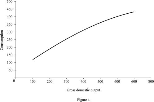
In Figure 4, the horizontal axis measures the gross domestic output and the vertical axis measures the consumption level.
Concept introduction:
Consumption schedule: Consumption schedule refers to the quantity of consumption at different levels of income.
Marginal propensity to consume (MPS): Marginal propensity to consume refers to the sensitivity of change in the consumption level due to the changes occurred in the income level.
Multiplier: Multiplier refers to the ratio of change in the real GDP to the change in initial consumption at constant price rate. Multiplier is positively related to the marginal propensity to consumer and negatively related with the marginal propensity to save.
Sup part (e):
Marginal propensity to consume and multiplier.
Sup part (e):
Explanation of Solution
Figure 1, Figure 2, Figure 3 and Figure 4 reveals that the proportional and progressive tax system reduces the value of MPC, so that the value of multiplier also decreases. The regressive tax system (Lump sum tax) does not alter the MPC. Since there is no change in the MPC, the multiplier remains the same.
Concept introduction:
Marginal propensity to consume (MPS): Marginal propensity to consume refers to the sensitivity of change in the consumption level due to the changes occurred in the income level.
Progressive tax: Progressive tax refers to the higher income people paying higher tax amount than the lower income people.
Proportional tax: Proportional tax rate refers to the fixed tax rate regardless of income and the tax rate and is the same for all levels of income.
Regressive tax: Regressive tax refers to the higher income people paying lower percentage of tax amount and lower income people paying higher percentage of tax amount.
Multiplier: Multiplier refers to the ratio of change in the real GDP to the change in initial consumption at constant price rate. Multiplier is positively related to the marginal propensity to consumer and negatively related with the marginal propensity to save.
Want to see more full solutions like this?

- 7 Real expenditure in thousands of dollars 6 5 3 2 0 1 Reference: Figure 10-5 O 0.25 O.0.50 2 O 0.75 Refer to the graph above. The mpe equals: O 1.00 3 4 5 6 7 Real income in thousands of dollars AE curvearrow_forwardAn economy has a consumption function of C = 20 + 0.75(YD), taxes = 10+0.2(Y), investment equal to 10, government expenditure equal to 15, exports equal to 15, and an import function of M = 10. 1) What is the equilibrium real GDP for this economy? O A. 156.25 O B. 146.88 Oc. 106.25 O D. 150.50 2) What is the multiplier for a change in government spending for this economy? O A. 3.5 O B. 2.5 O c. 3.0 O D. 4.0arrow_forwardAssume a closed economy, that taxes are fixed, and the marginal propensity to consume is equal to 0.66. What is the government spending multiplier? O 1.51 3.33 3.03 33.3arrow_forward
- Figure: Aggregate Expenditures Curve II Aggregate expenditures (per year) $800 Reference: Ref 11-16 45-degree line AE $2,000 Real GDP (per year) (Figure: Aggregate Expenditures Curve II) The slope of the aggregate expenditures curve in the aggregate expenditures model shown in this figure is: O 45 degrees. O 0.6. O 0.5. O 0.25.arrow_forwardIf government spending rises by $100, mps = 0.2, then the GDP multiplier is O 5 O 4 O 1arrow_forwardThe city of Joslyn has three sources of revenue: borrowing, proprietary income from running the local electric power utility, and taxes. Last year, its total revenue was $150 million. If it received $10 million from running the electric power utility and borrowed $40 million, how much did it collect in taxes? Assume Joslyn's total revenue is $150 million. O $100 million O $110 million O $140 million O Nothingarrow_forward
- QUESTION 10 Assuming that the "equilibrium income" is $4,000 and the "full-employment" income is $8,000, which means a recessionary gap of $4,000, how much change in government expenditures is needed to fill the gap if MPC is 0.50? O $3,000 O $4,000 O $1,000 O $2,000arrow_forwardReal GDP Consumption (dollars) expenditure (dollars) 10 22.5 20 30 30 37.5 40 45 50 52.5 60 60 2 LAS 160 * SAS 150 140 130 120 AD 4 8 12 16 20 24 Real GDP (trillions of 2000 dollars) In the above table and figure, supposed that there is no import or proportional tax. To pull the economy back to the long-run equilibrium, the government can conduct a balanced budget operation by spending $ trillion. O 1) 1 O 2) 2 O 3) 4 4) 8 el (GDP deflator, 2000 = 100) Coarrow_forward5. Refer to the data in the table that accompanies problem 2. Suppose that the present equilibrium price level and level of real GDP are 100 and $225, and that data set B represents the relevant aggregate supply schedule for the economy. LO12.6 a. What must be the current amount of real output demanded at the 100 price level? b. If the amount of output demanded declined by $25 at the 100 price level shown in B, what would be the new equilibrium real GDP? In business суcle economists call this change in real terminology, what would GDP?arrow_forward
- LAST WORD What is Say's law? How does it relate to the view held by classical economists that the economy generally will operate at a position on its production possibilities curve? Use production possibilities analysis to demonstrate Keynes's view on this matter.arrow_forwardRefer to the Table. The government spending multiplier in this economy is Planned Output (Income) Taves Consumption Savings Investment 1000 L100 Net Planned 200 680 120 200 200 140 200 200 1,200 200 200 200 840 160 1300 1400 1.500 920 200 200 200 LORO 200 1600 1,160 240 2. 4. 5. 10.arrow_forward5. LO 2,5 A consumer receives income y in the current period and income y' in the future period, and pays taxes of t and t' in the current and future periods, respectively. The consumer can borrow and lend at the real interest rate r. This consumer faces a constraint on how much he or she can borrow, much like the credit limit typically placed on a credit card account. That is, the consumer cannot borrow more than x, where x < we-y+t, with we denoting lifetime wealth. Use diagrams to determine the effects on the consumer's current consumption, future consumption, and saving of a change in x, and explain your results.arrow_forward

 Principles of Economics (12th Edition)EconomicsISBN:9780134078779Author:Karl E. Case, Ray C. Fair, Sharon E. OsterPublisher:PEARSON
 Engineering Economy (17th Edition)EconomicsISBN:9780134870069Author:William G. Sullivan, Elin M. Wicks, C. Patrick KoellingPublisher:PEARSON
 Principles of Economics (MindTap Course List)EconomicsISBN:9781305585126Author:N. Gregory MankiwPublisher:Cengage Learning
 Managerial Economics: A Problem Solving ApproachEconomicsISBN:9781337106665Author:Luke M. Froeb, Brian T. McCann, Michael R. Ward, Mike ShorPublisher:Cengage Learning
 Managerial Economics & Business Strategy (Mcgraw-...EconomicsISBN:9781259290619Author:Michael Baye, Jeff PrincePublisher:McGraw-Hill Education