To show:
The graphical representation of
Explanation of Solution
Average Cost function plays a pivotal role in establishing economies and diseconomies of scale.
Before the automation process and the assembly line production, cost of production of an automobile was exorbitant. This is shown in Panel a) of Figure 1. There were only few firms producing automobiles. Hence, their supply was limited. Average total cost of production curve AC shows the cost of Q1 of automobiles to be A1.
This cost reflects the average cost in 1901 when the technique of production to be used was limited and there were unspecialized workers. With assembly line production, division of labor was achieved. Automobile manufacturers were able to use specialized labor for specific activity. This greatly helped them in achieving economic of scale that reduced average cost of production.
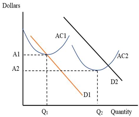
With time, there has been more use of machines that have replaced labor. This has reduced the per vehicle cost further down. This is shown by average total cost of production curve AC that shows the cost of Q2 units of automobiles to be A2 in Figure 1.
The demand curve for automobiles in 1901 was low, shown by D1 in Figure 1.People had limited financial sources to buy an automobile. Hence, they demanded fewer automobiles. With already limited supply of automobiles, the price was quite high.
By 2016, the prices have fallen because cost of production has reduced dramatically. Also, the income levels have increased for most of the consumers. This has increased their willingness to pay. Hence, the demand curve for automobiles in 2016 is higher and is shown as D2 in Figure 1.
Average Total Cost:
Average total cost is expressed as the cost incurred by the firm on the production of one unit of the output, on average. It can be measured from the total cost function when the latter is divided by the number of units produced.
Want to see more full solutions like this?
Chapter 18 Solutions
Foundations of Economics (8th Edition)

- Giocattolo is a profit-maximizing firm producing toy cars, which it can produce and sell in its home country, Italy, and abroad in Spain. The average cost (AC) curve on the following graph represents Giocattolo's cost of producing toy cars within one factory, whether in Italy or in Spain. COST (Dollars per toy car) 10 1 0 10 I 1 20 30 40 50 60 70 80 QUANTITY (Thousands of toy cars) AC 90 100 Suppose that at the current market price of toy cars, the demand for Giocattolo's product is 10,000 toy cars per year in Italy and 20,000 toy cars per year in Spain. (Hint: Select each point on the previous graph to see its coordinates.) (?) Based on Giocattolo's average cost curve, within one factory it can produce 20,000 toy cars at S per toy car, and produce the total of 30,000 toy cars at S per toy car. Complete the following table by indicating Giocattolo's total production cost for each scenario. Total Production Cost (Dollars) Scenario Produce 10,000 toy cars in Italy and 20,000 toy cars in…arrow_forwardSuppose Larry runs a small business that manufactures shirts. Assume that the market for shirts is a price-taker market, and the market price is $10 per shirt. The following graph shows Larry's total cost curve. Use the blue points (circle symbol) to plot total revenue and the green points (triangle symbol) to plot profit for the first seven shirts that Larry produces, including zero shirts. 125 100 TOTAL COST AND REVENUE (Dollars) 25 ☐ Total Cost ☐ -50 0 1 2 3 4 5 6 7 8 QUANTITY (Shirts) Total Revenue A Profit (?) Calculate Larry's marginal revenue and marginal cost for the first seven shirts he produces and plot them on the following graph. Use the blue points (circle symbol) to plot marginal revenue and the orange points (square symbol) to plot marginal cost. 25 2 COSTS AND REVENUE (Dollars per shirt) 0 1 2 3 5 6 7 8 QUANTITY (Shirts) Marginal Revenue Marginal Cost Larry's profit is maximized when he produces is shirts. When he does this, the marginal cost of the previous shirt he…arrow_forwardQuestions 1-3 use the following case to determine a way to take a single product, like toilet and bundle it in such a way as to extract all of the profit at the time of the initial sale. You go to CostCo or Walmart and you see paper towel sold in a bundle and you wonder how the retailer can make any money. You do a little research and you find that the demand for paper towels is depicted by the following demand curve and marginal cost: P=$2.20 (1/10)*Q MR-$2.20 (2/10)*Q MC 0.20 where P is the price of paper towels, MC is the marginal cost of paper towels, MR is the marginal revenue of paper towels and Q is the quantity of paper towels. So you decide to try two different pricing strategies: 1) sell one roll at a time and 2) use multipart pricing to sell a bundle. Given the results for the pricing strategies in problems 1 and 2, what is your pricing decision and why?arrow_forward
- The graph shows the demand curve for cars in 2017. Suppose that the least-possible cost of producing a car is $10,000 and that the efficient scale is 10,000 cars a month. Draw the average total cost curve for a car manufacturer in 2017. Label it. 50,000 40,000- 30,000 20,000 10,000- Price (dollars per car) D 20 30 40 10 Quantity (thousands of cars per month) >>> Draw only the objects specified in the question. Q OUarrow_forwardThe following graph illustrates the weekly demand curve for motorized scooters in Scottsdale. Use the green rectangle (triangle symbols) to compute total revenue at various prices along the demand curve. Note: You will not be graded on any changes made to this graph. PRICE (Dollars per scooter) TOTAL REVENUE (Dollars) 8700 8100 7500 6900 6300 5700 5100 4500 3900 325 3300 300 275 250 225 200 175 150 125 100 75 On the following graph, use the green point (triangle symbol) to plot the weekly total revenue when the market price is $50, $75, $100, $125, $150, $175, and $200 per scooter. (?) 50 25 0 0 10 20 *4 0 25 50 Xo Demand 30 40 50 60 70 80 90 100 110 120 130 QUANTITY (Scooters) Total Revenue 75 100 125 150 175 200 225 250 275 300 325 PRICE (Dollars per scooter) (?) Total Revenue According to the midpoint method, the price elasticity of demand between points A and B is approximatelyarrow_forwardThe table below presents the average and marginal cost of producing cheeseburgers per hour at a roadside diner. Cheeseburger Production Costs Quantity(burgers per hour) Average Variable Cost (dollars) Average Total Cost (dollars) Marginal Cost (dollars) 0 — — — 10 $1.00 $6.60 $1.00 20 0.70 3.50 0.40 30 0.70 2.57 0.70 40 0.78 2.18 1.00 50 0.88 2.00 1.30 60 1.07 2.00 2.00 70 1.34 2.14 3.00 80 1.74 2.44 4.50 90 2.23 2.86 6.20 100 2.81 3.37 8.00 a. At a quantity of 40 cheeseburgers per hour, the average total cost of production is (Click to select) falling rising at a minimum and the marginal cost of cheeseburger production is (Click to select) falling rising at a minimum . b. At a quantity of 60 cheeseburgers per hour, the average variable cost of production is (Click to select) falling rising at a minimum and the average total cost of cheeseburger production is (Click to select) falling rising at a minimum .arrow_forward
- The following table represents the demand schedule (given by the first two columns of the table), TC, MC, TR and MR for one of many landscaping companies in Florida. The service the company provides includes mowing, planting some flowers and trimming trees. Use the information from the table to answer the questions below. The goal of the landscaping company is to maximize its profit. How many customers should it serve per day? What price should it charge? How much profit does this company make per day if it is maximizing its profit?arrow_forwardIf Amit's Curry House took in $35 000 in revenue last week and had out-of-pocket expenses of $31 500, which of the following best describes Amit's profits last week? Amit really did NOT make any profit since he needs to put the difference between revenue and out-of-pocket expenses back into the firm. Amit made an economic profit of $3500. It is NOT clear whether Amit earned any profit last week because it depends on the magnitude of the implicit costs. Amit did NOT earn an economic profit.arrow_forwardAssume you are selling season tickets for a team in the National Football League. What are the fixed and variable costs associated with pricing these season tickets? When you look at the existing season ticket prices for the team, how would you sell those same season tickets at a 10 percent higher price?arrow_forward
- Increasing demand from China has made New Zealand the world's biggest exporter of dairy products . Its exports of milk to China increased by 45 % in 2013. More than 300 000 hectares land in New Zealand have been transferred to dairy use from other forms of farming and forestry use since 2000. The increase in milk production has caused the average cost of its production to fall and changes in production methods have affected the price elasticity of supply of milk . Discuss whether the average cost of production always decreases when a firm increases the total output that it produces(Define economies of scale and diseconomies of scale Use of graph to explain ( if applicable ) Explain the various economies of scale e.g. purchasing economies of scale [ up to 5 ] Explain the various diseconomies of scale [ up to Brief conclusion)arrow_forwardSuppose Felix runs a small business that manufactures frying pans. Assume that the market for frying pans is a competitive market, and the market price is $20 per frying pan. The following graph shows Felix's total cost curve. Use the blue points (circle symbol) to plot total revenue and the green points (triangle symbol) to plot profit for frying pans quantities zero through seven (inclusive) that Felix produces. TOTAL COST AND REVENUE (Dollars) 200 175 150 125 100 75 50 25 0 -25 0 1 ● ^ 2 O ☐ A ☐ A 3 4 5 QUANTITY (Frying pans) O ☐ 6 Total Cost ☐ 7 8 o Total Revenue Profit ? image 1 Calculate Felix's marginal revenue and marginal cost for the first seven frying pans he produces, and plot them on the following graph. Use the blue points (circle symbol) to plot marginal revenue and the orange points (square symbol) to plot marginal cost at each quantity.arrow_forwardSuppose the imaginary company of Roobek is a small, Reno-based American apparel manufacturer specializing in athleisure. The following table presents the brand’s total cost of production at several different quantities. Fill in the remaining cells of the following table. Quantity Total Cost Marginal Cost Fixed Cost Variable Cost Average Variable Cost Average Total Cost (Pairs) (Dollars) (Dollars) (Dollars) (Dollars) (Dollars per pair) (Dollars per pair) 0 60 — — 1 160 2 220 3 270 4 340 5 450 6 630 On the following graph, plot Douglas Fur’s average total cost (ATC) curve using the green points (triangle symbol). Next, plot its average variable cost (AVC) curve using the purple points (diamond symbol). Finally, plot its marginal cost (MC) curve using the orange points (square symbol). (Hint: For ATC…arrow_forward
 Microeconomics: Principles & PolicyEconomicsISBN:9781337794992Author:William J. Baumol, Alan S. Blinder, John L. SolowPublisher:Cengage Learning
 Managerial Economics: A Problem Solving ApproachEconomicsISBN:9781337106665Author:Luke M. Froeb, Brian T. McCann, Michael R. Ward, Mike ShorPublisher:Cengage Learning

