Concept explainers
Videos
Expand Your Knowledge: Residual Plot The least-squares line usually does not go through all the sample data points (x, y). In fact, for a specified x value from a data pair (x, y), there is usually a difference between the predicted value and the y value paired with x. This difference is called the residual.
The residual is the difference between the y value in a specified data pair (x, y) and the value
One way to assess how well a least-squares line serves as a model for the data is a residual plot. To make a residual plot, we pull the x values in order on the horizontal axis and plot the corresponding residuals
| Residual | |||||||
| X | y |
|
|
||||
| 6 | 15 | 12.6 | 2.4 | ||||
| 20 | 31 | 26.8 | 4.2 | ||||
| 0 | 10 | 6.6 | 3.4 | ||||
| 14 | 16 | 20.7 | -4.7 | ||||
| 25 | 28 | 31.8 | -3.8 | ||||
| Residual | |||||||
| X | y |
|
|
||||
| 16 | 20 | 22.7 | -2.7 | ||||
| 28 | 40 | 34.8 | 5.2 | ||||
| 18 | 25 | 24.7 | 0.3 | ||||
| 10 | 12 | 16.7 | -4.7 | ||||
| 8 | 15 | 14.6 | 0.4 | ||||
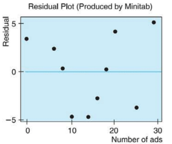
If the least-squares line provides a reasonable model for the data, the pattern of points in the plot will seem random and unstructured about the horizontal line at 0. Is this the case for the residual plot?
If a point on the residual plot seems far outside the pattern of other points, it might reflect an unusual data point (x. y), called an outlier. Such points may have quite an influence on the least-squares model. Do there appear to be any outliers in the data for the residual plot?

Trending nowThis is a popular solution!

Chapter 4 Solutions
Understanding Basic Statistics


- If your graphing calculator is capable of computing a least-squares sinusoidal regression model, use it to find a second model for the data. Graph this new equation along with your first model. How do they compare?arrow_forwardBeachcomer Ltd is a local car dealership that sells used and new vehicles. The manager of the company wants to know how different variables affect the sales of his vehicles. A random sample of yearly data was taken with the view to testing the model. SALES = a+BAGE + yMIL + SENG Where SALES = amount that a vehicle is sold for (000's), AGE = age of vehicle, MIL= the total mileage of the vehicle at the point of sale and ENG = the size of the engine. The sample of data was processed using MINITAB and the following is an extract of the output obtained: The regression equation is ***** Coef StDev t-ratio p-value Predictor Constant 1.7586 0.2525 6.9648 0.0000 AGE 0.2124 0.3175 * 0.5042 MIL -0.7527 0.3586 -2.0991 ** ENG 4.8124 0.6196 7.7664 0.0000…arrow_forwardBeachcomer Ltd is a local car dealership that sells used and new vehicles. The manager of the company wants to know how different variables affect the sales of his vehicles. A random sample of yearly data was taken with the view to testing the model. SALES = a+BAGE + yMIL + SENG Where SALES = amount that a vehicle is sold for (000's), AGE = age of vehicle, MIL= the total mileage of the vehicle at the point of sale and ENG = the size of the engine. The sample of data was processed using MINITAB and the following is an extract of the output obtained: The regression equation is ***** Coef StDev t-ratio p-value Predictor Constant 1.7586 0.2525 6.9648 0.0000 AGE 0.2124 0.3175 * 0.5042 MIL -0.7527 0.3586 -2.0991 ** ENG 4.8124 0.6196 7.7664 0.0000…arrow_forward
- Beachcomer Ltd is a local car dealership that sells used and new vehicles. The manager of the company wants to know how different variables affect the sales of his vehicles. A random sample of yearly data was taken with the view to testing the model. SALES = a+BAGE + yMIL + SENG Where SALES = amount that a vehicle is sold for (000's), AGE = age of vehicle, MIL= the total mileage of the vehicle at the point of sale and ENG = the size of the engine. The sample of data was processed using MINITAB and the following is an extract of the output obtained: The regression equation is ***** Coef StDev t-ratio p-value Predictor Constant 1.7586 0.2525 6.9648 0.0000 AGE 0.2124 0.3175 * 0.5042 MIL -0.7527 0.3586 -2.0991 ** ENG 4.8124 0.6196 7.7664 0.0000…arrow_forwardTable gives life expectancies for people born in the United States in the given years. (a) Determine the least squares approximating line for these data and use it to predict the life expectancy of someone born in 2000. (b) How good is this model? Explain.arrow_forwardBeachcomer Ltd is a local car dealership that sells used and new vehicles. The manager of the company wants to know how different variables affect the sales of his vehicles. A random sample of yearly data was taken with the view to testing the model. SALES = a+BAGE + yMIL + SENG Where SALES = amount that a vehicle is sold for (000's), AGE = age of vehicle, MIL= the total mileage of the vehicle at the point of sale and ENG = the size of the engine. The sample of data was processed using MINITAB and the following is an extract of the output obtained: The regression equation is ***** Coef StDev t-ratio p-value Predictor Constant 1.7586 0.2525 6.9648 0.0000 AGE 0.2124 0.3175 * 0.5042 MIL -0.7527 0.3586 -2.0991 ** ENG 4.8124 0.6196 7.7664 0.0000…arrow_forward
- Which equation is the best fit for the data in the table? X Y 3 12 5 27 8 48 11 O y=-.0026x^2+.33x+1.16 O y=1.94x+2.140 O y=1.732vx-1 O y=1.732x-1arrow_forwardPlease help me to write the interpretation for ANOVA and linear regression for both countries in Austria and United Kingdom (Attachment is there)arrow_forwardHow can one locate mode graphically in case of grouped data?arrow_forward
 Algebra & Trigonometry with Analytic GeometryAlgebraISBN:9781133382119Author:SwokowskiPublisher:Cengage
 Trigonometry (MindTap Course List)TrigonometryISBN:9781305652224Author:Charles P. McKeague, Mark D. TurnerPublisher:Cengage Learning
 Glencoe Algebra 1, Student Edition, 9780079039897...AlgebraISBN:9780079039897Author:CarterPublisher:McGraw Hill
 Big Ideas Math A Bridge To Success Algebra 1: Stu...AlgebraISBN:9781680331141Author:HOUGHTON MIFFLIN HARCOURTPublisher:Houghton Mifflin Harcourt
 Holt Mcdougal Larson Pre-algebra: Student Edition...AlgebraISBN:9780547587776Author:HOLT MCDOUGALPublisher:HOLT MCDOUGAL