
Videos
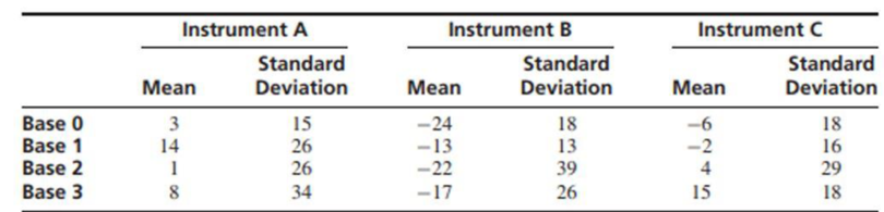
The article “Combined Analysis of Real-Time Kinematic GPS Equipment and Its Users for Height Determination” (W. Featherstone and M. Stewart, Journal of Surveying Engineering. 2001:31–51) presents a study of the accuracy of global positioning system (GPS) equipment in measuring heights. Three types of equipment were studied, and each was used to make measurements at four different base stations (in the article a fifth station was included, for which the results differed considerably from the other four). There were 60 measurements made with each piece of equipment at each base. The means and standard deviations of the measurement errors (in mm) are presented in the following table for each combination of equipment type and base station.
- a. Construct an ANOVA table. You may give
ranges for the P-values. - b. The question of interest is whether the mean error differs among instruments. It is not of interest to determine whether the error differs among base stations. For this reason, a surveyor suggests treating this as a randomized complete block design, with the base stations as the blocks. Is this appropriate? Explain.
a.
Construct the ANOVA.
Answer to Problem 9SE
The ANOVA table is,
| Source | DF | SS | MS | F | P |
| Base | 3 | 13,495 | 4498.3 | 7.5308 | 0.000 |
| Instrument | 2 | 90,990 | 45,495 | 76.164 | 0.000 |
| Interaction | 6 | 12,050 | 2,008.3 | 3.3622 | 0.003 |
| Error | 708 | 422,912 | 597.33 | ||
| Total | 719 | 539,447 |
Explanation of Solution
Calculation:
The given information is based on the accuracy of the global positioning system (GPS) which has 3 instruments that have to make measurements at four different base stations have 60 measurements with each piece of instrument at each base.
Let us denote the main effects of Instruments (I) with
The aim is to find the ANOVA.
State the hypothesis:
Main effect of Instruments:
Null hypothesis:
Alternative hypothesis:
Main effect of Base:
Null hypothesis:
Alternative hypothesis:
Interaction:
Null hypothesis:
Alternative hypothesis:
ANOVA table:
| Source | DF | SS | MS | F |
| Treatment | ||||
| Blocks | ||||
| Interaction | ||||
| Error | ||||
| Total |
Where,
Where, N is the sample size, I denotes the number of treatments,
Here, the number of treatments (I) is 3, the number of blocks (J) is 4 and the number of replicates (K) is 60.
Test the hypothesis on 5% level of significance:
Here, Instrument is the treatments and Base is the blocks.
Level of significance:
The level of significance is
Degrees of freedom:
Base degrees of freedom:
Instrument degrees of freedom:
Interaction degrees of freedom:
Error degrees of freedom:
Total degrees of freedom:
The treatment and block means are tabulated below:
| Base | Instruments | Block mean | ||
| Instrument A | Instrument B | Instrument C | ||
| 0 | 3 | –24 | –6 | –9 |
| 1 | 14 | –13 | –2 | –0.33 |
| 2 | 1 | –22 | 4 | –5.667 |
| 3 | 8 | –17 | 15 | 2 |
| Treatment mean | 6.5 | –19 | 2.75 | |
By observing the data, the values of
For Base:
The value of SSB (Base) is:
Substitute
The value of MSB (Base) is:
Substitute
For Instruments:
The value of SSTr ( Instruments) is:
Substitute
The value of MSTr (Instruments) is:
Substitute
For Interaction Factor (AB):
The value of SSAB is:
Substitute
The value of MSAB is:
Substitute
The value of MSE is:
Substitute
The value of SSE is:
The value of SST is:
The value of F statistic is:
For Base:
Substitute
Thus, the value of F statistic for Base is 7.5308.
For Instruments:
Substitute
Thus, the value of F statistic for Instruments is 76.164.
For Interaction factor (AB):
Substitute
Thus, the value of F statistic for interaction is 3.3622.
The ranges of P-values are:
For Base
Software procedure:
Step by step procedure to obtain the critical-value using the MINITAB software is given below:
- Choose Graph > Probability Distribution Plot choose View Probability> OK.
- From Distribution, choose ‘F’ distribution.
- Enter Numerator Df as 3.
- Enter Denominator Df as 708.
- Click the Shaded Area tab.
- Choose X Value and Right Tail for the region of the curve to shade.
- Enter the Data value as 7.5308.
- Click OK.
Output using the MINITAB software is given below:
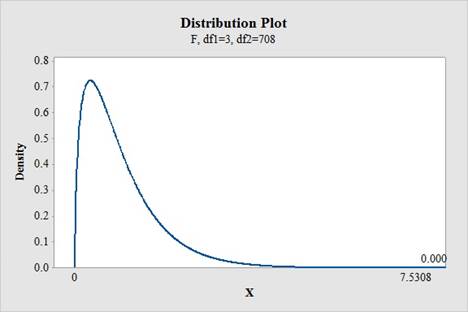
From the MINITAB output, the value of
For Instruments
Software procedure:
Step by step procedure to obtain the critical-value using the MINITAB software is given below:
- Choose Graph > Probability Distribution Plot choose View Probability> OK.
- From Distribution, choose ‘F’ distribution.
- Enter Numerator Df as 2.
- Enter Denominator Df as 708.
- Click the Shaded Area tab.
- Choose X Value and Right Tail for the region of the curve to shade.
- Enter the Data value as 76.164.
- Click OK.
Output using the MINITAB software is given below:
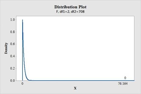
From the MINITAB output, the value of
For interaction
Software procedure:
Step by step procedure to obtain the critical-value using the MINITAB software is given below:
- Choose Graph > Probability Distribution Plot choose View Probability> OK.
- From Distribution, choose ‘F’ distribution.
- Enter Numerator Df as 6.
- Enter Denominator Df as 708.
- Click the Shaded Area tab.
- Choose X Value and Right Tail for the region of the curve to shade.
- Enter the Data value as 3.3622.
- Click OK.
Output using the MINITAB software is given below:
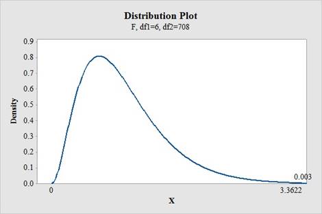
From the MINITAB output, the value of
The ANOVA table is,
| Source | DF | SS | MS | F | P |
| Base | 3 | 13,495 | 4498.3 | 7.5308 | 0.000 |
| Instrument | 2 | 90,990 | 45,495 | 76.164 | 0.000 |
| Interaction | 6 | 12,050 | 2,008.3 | 3.3622 | 0.003 |
| Error | 708 | 422,912 | 597.33 | ||
| Total | 719 | 539,447 |
Conclusion:
Base (Block):
Here, the P-value is less than the level of significance.
That is,
Therefore, the null hypothesis is rejected.
Thus, it can be concluded that there is a significant difference between block effects.
Instrument (Treatment):
Here, the P-value is less than the level of significance.
That is,
Therefore, the null hypothesis is rejected.
Thus, it can be concluded that there is a significant difference between treatment effects.
Interaction:
Here, the P-value is less than the level of significance.
That is,
Therefore, the null hypothesis is rejected.
Thus, it can be concluded that there is a significant effect of the interaction between the base (block) and instrument (treatment).
b.
Decide whether it is appropriate to treat the randomized complete block design with base stations as blocks to determine the interest that the mean error differs among the instruments.
Answer to Problem 9SE
No, it is not appropriate to treat the data with a randomized complete block design with base stations as blocks.
Explanation of Solution
In randomized complete block design, there must be no the interaction between the treatment factor and the blocking factor, so that the treatment factor may be interpreted in RBD. However, here, the interaction effect is significant, suggesting that it is not possible to use randomized complete block design.
Thus, the suggestion given by the surveyor to treat the randomized complete block design with base station as blocks is not appropriate.
Want to see more full solutions like this?
Chapter 9 Solutions
Statistics for Engineers and Scientists
Additional Math Textbook Solutions
Statistical Techniques in Business and Economics
Fundamentals of Statistics (5th Edition)
Statistical Reasoning for Everyday Life (5th Edition)
An Introduction to Mathematical Statistics and Its Applications (6th Edition)
APPLIED STAT.IN BUS.+ECONOMICS
Elementary Statistics (13th Edition)


- 3. Load the Santa Barbara temperature data using the following com- mands stbarb=read.table ("berkeley.dat")[,3] Since the data is non-stationary, we consider taking difference of stbarb. Create ACF and PACF plots for the differenced data. Do you have an opinion on possible models based only on these plots?arrow_forwardgiven this data, what will be the most appropriate way to present them?arrow_forwardThe authors of a paper compared two different instruments for measuring a person's capacity for breathing out air. (This measurement is helpful in diagnosing various lung disorders.) The two instruments considered were a Wright peak flow meter and a mini-Wright peak flow meter. Seventeen people participated in the study, and for each person air flow was measured once using the Wright meter and once using the mini-Wright meter. The Wright meter is thought to provide a better measure of air flow, but the mini-Wright meter is easier to transport and to use. Use of the mini-Wright meter could be recommended as long as there is not convincing evidence that the mean reading for the mini-Wright meter is different from the mean reading for Wright meter. For purposes of this exercise, you can assume that it is reasonable to consider the 17 people who participated in this study as representative of the population of interest. Data values from this paper are given in the accompanying table.…arrow_forward
- NW 6.12 CORPORATE SUSTAINABILITY OF CPA FIRMS. Corporate sustainability refers to business practices designed CORSUS around social and environmental considerations. Refer to the Business and Society (March 2011) study on the sustainability behaviors of CPA corporations, Exercise 2.23 (p. 59). Recall that the level of support for corporate sustainability (measured on a quantitative scale ranging from 0 to 160 points) was obtained for each in a sample of 992 senior managers at CPA firms. Higher point values indicate a higher level of support for sustainability. The accompanying StatCrunch printout gives a 99% confidence interval for the mean level of support for all senior managers at CPA firms. One sample T confidence interval: μ: Mean of variable 99% confidence interval results: Variable Sample Mean Std. Err. DF L. Limit U. Limit Support 67.75504 0.85314633 991 65.553241 69.95684 a. Locate the 99% confidence interval on the printout. b. Use the sample mean and standard deviation on the…arrow_forwardGender and Direction. In the paper “The Relation of Sex and Sense of Direction to Spatial Orientation in an Unfamiliar Environment” (Journal of Environmental Psychology, Vol. 20, pp. 17–28), J. Sholl et al. published the results of examining the sense of direction of 30 male and 30 female students. After being taken to an unfamiliar wooded park, the students were given a number of spatial orientation tests, including pointing to south, which tested their absolute frame of reference. To point south, the students moved a pointer attached to a 360◦ protractor. The absolute pointing errors, in degrees, for students who rated themselves with a good sense of direction (GSOD) and those who rated themselves with a poor sense of direction (PSOD) are provided on the WeissStats site. Can you reasonably apply the two-standard-deviations F-test to compare the variation in pointing errors between people who rate themselves with a good sense of direction and those who rate themselves with a poor…arrow_forwardWhich model—the one for parliaments or the one for ministries (or cabinets)—presented in the article has the greater explanatory power? How can you tell?arrow_forward
- 1. (Prob. 11-12, p. 438) An article in the Journal of Environmental Engineering (1989, Vol. 115(3), pp. 608–619) reported the results of a study on the occurrence of sodium and chloride in surface streams in central Rhode Island. The following data are chloride concentration y (in milligrams per liter) and roadway area in the watershed x (in percentage). y 4.4 6.6 9.7 10.6 10.8 10.9 0.19 0.15 0.57 0.70 0.67 0.63 y 11.8 12.1 14.3 14.7 15.0 17.3 0.47 0.70 0.60 0.78 0.81 0.78 y 19.2 23.1 27.4 27.7 31.8 39.5 0.69 1.30 1.05 1.06 1.74 1.62 a. Draw a scatter diagram of the data. Does a simple linear regression model seem appropriate here? b. Fit the simple linear regression model using the method of least squares. Find an estimate of o?. C. Estimate the mean chloride concentration for a watershed that has 1% roadway area. d. Find the fitted value corresponding to x = 0.47 and the associated residual.arrow_forward4.) A person's muscle mass is expected to decrease with age. To explore this relationship, a researcher randomly selected 10 persons from ages 40 to 79 years old and measured their muscle mass (unit). The result is as follows: X (age) Y (muscle mass) 71 64 43 67 56 73 68 56 76 65 82 91 100 68 87 73 78 80 65 84 Based on the given data, do the following: a) Plot the scatter diagram of the given data. [3pts] b) Obtain the regression line equation. [4pts] c) Estimate the muscle mass when age of the person is 60 years old. [3pts] 5.) Recognize how each shape has transformed. [2pts each] a.) b.) c.)arrow_forwardZhou and Vohs (2009) published a study showing that handling money reduces the perception of pain. In the experiment, a group of college students was told that they were participating in a manual dexterity study. Half of the students were given a stack of money to count and the other half got a stack of blank pieces of paper. After the counting task, the participants were asked to dip their hands into bowls of very hot water (122° F) and rate how uncomfortable it was. The following data show ratings of pain similar to the results obtained in the study. Counting Money Counting Paper 7 9 8 11 10 13 6 10 8 11 5 9 7 15 12 14 5 10 Convert the data from this problem into a form suitable for the point-biserial correlation (use Y = 1 for the money and 0 for the plain paper), and then compute the correlation. ∑X ∑Y ∑XY SSXX SSYY SP r Square the value of the point-biserial correlation to obtain r².…arrow_forward
- 4. 2. 2. 3. Express the varia If a truck were driven 80,000 KI expect to be incurred? Archer Company is a wholesaler of custom-built air-conditioning units for commercial buildings. It gathered the following monthly data relating to units shipped and total shipping expense: EXERCISE 5A-4 High-Low Method; Scattergraph Analysis LO5-10 Month January... February. March April.... May June.......**** July Units Shipped 3 6 4 5 7 8 2 Total Shipping Expense $1,800 $2,300 $1,700 $2,000 $2.300 $2.700 $1,200 Required: 1. Prepare a scattergraph using the data given above. Plot cost on the vertical axis and activity on the horizontal axis. Is there an approximately linear relationship between shipping expense and the number of units shipped? Cost-Volume-Profit Relationships Using the high-low method, estimate the cost formula for shipping expense. Draw a straight line through the high and low data points shown in the scattergraph you prepared in require- ment (1). Make sure your line intersects the…arrow_forwardHere are the world record race times for women in the 10,000-meter run over several years. a) Which is the explanatory variable and which is the response variable? Year Race Time (seconds) 1967 2286.4 b) Make a scatterplot of these data. You do not have to draw the scatterplot for me. Describe what you see (form, direction, 1970 2130.5 1975 2100.4 strength, outliers). 1975 2041.4 c) Write the equation of the regression line for predicting race time from year. 1977 1995.1 1979 1972.5 d) Give the meaning of the slope of your line in terms of race time and year. What are the units of the slope in this problem? 1981 1950.8 1981 1937.2 e) What percent of the observed variation in 1982 1895.3 the race times can be explained by your 1983 1895.0 model? 1983 1887.6 f) Find the residual for the first data point or 1984 1873.8 the list (the 2286.4 seconds from 1967). 1985 1859.4 g) What does this linear model predict for th race time in the year 2075? Do you think 1986 1813.7 this is reasonable?…arrow_forward6.7 (4) 7 The following three equations were estimated using the 1,534 observations in 401K.RAW: prate = 80.29 + 5.44 mrate + .269 age – .00013 totemp (.045) (.78) (.52) (.00004) R = .100, R² = .098. prate = 97.32 + 5.02 mrate + .314 age – 2.66 log(totemp) (1.95) (0.51) (.044) (.28) R? = .144, R² = .142. prate = 80.62 + 5.34 mrate + .290 age – .00043 totemp (.045) (.78) (.52) (.00009) + .0000000039 totemp? (.0000000010) R? = .108, R² = .106. Which of these three models do you prefer? Why?arrow_forward
 MATLAB: An Introduction with ApplicationsStatisticsISBN:9781119256830Author:Amos GilatPublisher:John Wiley & Sons Inc
 Probability and Statistics for Engineering and th...StatisticsISBN:9781305251809Author:Jay L. DevorePublisher:Cengage Learning
 Statistics for The Behavioral Sciences (MindTap C...StatisticsISBN:9781305504912Author:Frederick J Gravetter, Larry B. WallnauPublisher:Cengage Learning
 Elementary Statistics: Picturing the World (7th E...StatisticsISBN:9780134683416Author:Ron Larson, Betsy FarberPublisher:PEARSON
 The Basic Practice of StatisticsStatisticsISBN:9781319042578Author:David S. Moore, William I. Notz, Michael A. FlignerPublisher:W. H. Freeman
 Introduction to the Practice of StatisticsStatisticsISBN:9781319013387Author:David S. Moore, George P. McCabe, Bruce A. CraigPublisher:W. H. Freeman